Migrating to AiiDA
Contents
3. Migrating to AiiDA#
Learning Objectives
In this section, we will look at how to migrate from running a quantum code from text-based input files, to running it within AiiDA, and understand how AiiDA automates the computation execution and output parsing.
We shall take the example of Quantum ESPRESSO, but the same principles apply to any other code. This would be a typical command line script to run a Quantum ESPRESSO relaxation:
$ mpirun -np 2 pw.x -in pwx.in > pwx.out
3.1. Modularising the inputs#
The first step is to modularise the inputs within the input.in file, and any pseudo-potential files.
By splitting them into separate components, we can create re-usable building blocks for multiple calculations. We shall also see later how these components can be generated from external data sources, such as databases or web APIs.

In the diagram above, we have split the input generation into separate entities, handling the different aspects of the calculation and allowing for component re-use.
For a pw.x calculation, we need to create the following nodes:
Computer, which describes how we interface with a compute resource
Code, which contains the information on how to execute a single calculation
StructureData, which contains the crystal structureUpfData, which contains the pseudo-potentials per atomicKpointsData, which contains the k-point meshDictnode, which contains the parameters for the calculation
3.2. The AiiDA Profile#
First we need to create a new AiiDA profile. This is where we store all the nodes generated for a project, and the links between them.
Note
Here we generate a profile with temporary, in-memory storage, which will be destroyed when the Python is restarted.
This is useful for testing, but for a real project, you would create a persistent profile connected to a PostgreSQL database,
using the verdi quicksetup command.
Show cell content
from local_module import load_temp_profile

data = load_temp_profile(name="qe-to-aiida")
data
AiiDALoaded(profile=Profile<uuid='6f7a7f8cd5b245d9a77f199beb7970a1' name='qe-to-aiida'>, computer=None, code=None, pseudos=None, structure=None, cpu_count=1, workdir=PosixPath('/home/docs/checkouts/readthedocs.org/user_builds/aiida-qe-demo/checkouts/latest/tutorial/local_module/_aiida_workdir/qe-to-aiida'), pwx_path=PosixPath('/home/docs/checkouts/readthedocs.org/user_builds/aiida-qe-demo/conda/latest/bin/pw.x'))
import aiida

profile = aiida.load_profile("qe-to-aiida")
profile
Profile<uuid='6f7a7f8cd5b245d9a77f199beb7970a1' name='qe-to-aiida'>
%verdi profile show qe-to-aiida
Report: Profile: qe-to-aiida
PROFILE_UUID: 6f7a7f8cd5b245d9a77f199beb7970a1
default_user_email: user@email.com
options:
  runner.poll.interval: 1
process_control:
  backend: 'null'
  config: {}
storage:
  backend: sqlite_temp
  config:
    debug: false
    repository_uri: file:///home/docs/checkouts/readthedocs.org/user_builds/aiida-qe-demo/checkouts/latest/tutorial/local_module/_aiida_path/.aiida/repository/qe-to-aiida
We can check on the status of the profile using the verdi status command.
%verdi -p qe-to-aiida status --no-rmq
 ✔ version:     AiiDA v2.0.4
 ✔ config:      /home/docs/checkouts/readthedocs.org/user_builds/aiida-qe-demo/checkouts/latest/tutorial/local_module/_aiida_path/.aiida
 ✔ profile:     qe-to-aiida
 ✔ storage:     SqliteTemp storage [open], sandbox: /home/docs/checkouts/readthedocs.org/user_builds/aiida-qe-demo/checkouts/latest/tutorial/local_module/_aiida_path/.aiida/repository/qe-to-aiida
 ⏺ daemon:      The daemon is not running
We can also check the statistics of the profile’s storage. Before running any simulations, we see that only a single User node has been created, which is the default creator of data for the profile.
%verdi storage info
entities:
  Users:
    count: 1
  Computers:
    count: 0
  Nodes:
    count: 0
  Groups:
    count: 0
  Comments:
    count: 0
  Logs:
    count: 0
  Links:
    count: 0
3.3. Connecting to a compute resource#
An AiiDA Computer represents a compute resource, such as a local or remote machine. It contains information on how to connect to the machine, how to transport data to/from the compute resource, and how to schedule jobs on it.
In the following we will use a simple local_direct computer, which connects to the local machine, and runs the calculations directly, without any scheduler.
AiiDA also has built-in support for a number of Schedulers, including:
pbsproslurmsgetorquelsf
Connections to remote machines can be made using the SSH Transport, and aiida-code-registry provides a collection of example configurations for Swiss based HPC clusters.
We can create the computer using the verdi computer setup CLI.
%verdi computer setup \
    --non-interactive \
    --label local_direct \
    --hostname localhost \
    --description "Local computer with direct scheduler" \
    --transport core.local \
    --scheduler core.direct \
    --work-dir {data.workdir} \
    --mpiprocs-per-machine {data.cpu_count}
Success: Computer<1> local_direct created
Report: Note: before the computer can be used, it has to be configured with the command:
Report:   verdi -p qe-to-aiida computer configure core.local local_direct
%verdi computer configure core.local local_direct \
    --non-interactive \
    --safe-interval 0
Report: Configuring computer local_direct for user user@email.com.
Success: local_direct successfully configured for user@email.com
Or we can use the Computer class from the aiida.orm API module.
created, computer = aiida.orm.Computer.collection.get_or_create(
    label="local_direct",
    description="local computer with direct scheduler",
    hostname="localhost",
    workdir=str(data.workdir),
    transport_type="core.local",
    scheduler_type="core.direct",
)
if created:
    computer.store()
    computer.set_minimum_job_poll_interval(0.0)
    computer.set_default_mpiprocs_per_machine(data.cpu_count)
    computer.configure()
computer
<Computer: local_direct (localhost), pk: 1>
Now we have a computer, ready to run calculations on.
%verdi computer show local_direct
---------------------------  --------------------------------------------------------------------------------------------------------------------------------
Label                        local_direct
PK                           1
UUID                         26ea091d-e317-4b9b-97a8-b01f2ddb274c
Description                  Local computer with direct scheduler
Hostname                     localhost
Transport type               core.local
Scheduler type               core.direct
Work directory               /home/docs/checkouts/readthedocs.org/user_builds/aiida-qe-demo/checkouts/latest/tutorial/local_module/_aiida_workdir/qe-to-aiida
Shebang                      #!/bin/bash
Mpirun command               mpirun -np {tot_num_mpiprocs}
Default #procs/machine       1
Default memory (kB)/machine
Prepend text
Append text
---------------------------  --------------------------------------------------------------------------------------------------------------------------------
3.4. Setting up a code plugin#
An AiiDA Code represent a single executable, and contain information on how to execute it.
The Code node is associated with a specific Computer, contains the path to the executable, and is associated with a specific CalcJob plugin we shall discuss later.
Again, we can use either the CLI or the API to create a new Code node.
%verdi code setup \
    --non-interactive \
    --label pw.x \
    --description "Quantum ESPRESSO pw.x code" \
    --computer local_direct \
    --remote-abs-path {data.pwx_path} \
    --input-plugin quantumespresso.pw \
    --prepend-text "export OMP_NUM_THREADS=1"
Success: Code<1> pw.x@local_direct created
try:
    code = aiida.orm.load_code("pw.x@local_direct")
except aiida.common.NotExistent:
    code = aiida.orm.Code(
        input_plugin_name="quantumespresso.pw",
        remote_computer_exec=[computer, data.pwx_path],
    )
    code.label = "pw.x"
    code.description = "Quantum ESPRESSO pw.x code"
    code.set_prepend_text("export OMP_NUM_THREADS=1")
    code.store()
code
<Code: Remote code 'pw.x' on local_direct, pk: 1, uuid: 2afdefc2-dd76-485e-a232-77ea9e5ac492>
Now we have a code ready to run our computations.
%verdi code show pw.x
--------------------  ------------------------------------------------------------------------------------
PK                    1
UUID                  2afdefc2-dd76-485e-a232-77ea9e5ac492
Label                 pw.x
Description           Quantum ESPRESSO pw.x code
Default plugin        quantumespresso.pw
Type                  remote
Remote machine        local_direct
Remote absolute path  /home/docs/checkouts/readthedocs.org/user_builds/aiida-qe-demo/conda/latest/bin/pw.x
Prepend text          export OMP_NUM_THREADS=1
Append text
--------------------  ------------------------------------------------------------------------------------
3.5. Deconstructing the input file#
Let’s now take a look at a typical pw.x input file, and how we can convert it to the requisite AiiDA nodes.
Note
Here we are simply generating the inputs from a pre-written input file. But in practice, you would want to generate the inputs from a Python script, or from a database or web API, as we shall see in the next section.
%cat direct_run/pwx.in
Show cell output
&CONTROL
  calculation = 'relax'
  etot_conv_thr =   2.0000000000d-04
  forc_conv_thr =   1.0000000000d-03
  max_seconds =   86400
  outdir = './out/'
  prefix = 'aiida'
  pseudo_dir = './pseudo/'
  restart_mode = 'from_scratch'
  tprnfor = .true.
  tstress = .true.
  verbosity = 'high'
/
&SYSTEM
  degauss =   1.0000000000d-02
  ecutrho =   2.4000000000d+02
  ecutwfc =   3.0000000000d+01
  ibrav = 0
  nat = 2
  nosym = .false.
  ntyp = 1
  occupations = 'smearing'
  smearing = 'cold'
/
&ELECTRONS
  conv_thr =   8.0000000000d-10
  electron_maxstep = 80
  mixing_beta =   4.0000000000d-01
/
&IONS
/
ATOMIC_SPECIES
Si     28.085 Si.pbe-n-rrkjus_psl.1.0.0.UPF
ATOMIC_POSITIONS angstrom
Si           0.0000000000       0.0000000000       0.0000000000
Si           1.8940738226       1.0935440313       0.7732524001
K_POINTS automatic
5 5 5 0 0 0
CELL_PARAMETERS angstrom
      3.7881476452       0.0000000000       0.0000000000
      1.8940738226       3.2806320940       0.0000000000
      1.8940738226       1.0935440313       3.0930096003
To decompose this file into the components we need, we can use the qe_tools package, which provides a Python API to parse Quantum ESPRESSO input files.
import qe_tools

pw_input = qe_tools.parsers.PwInputFile(open("direct_run/pwx.in").read())
pw_input
Show cell output
<qe_tools.parsers._pw_input.PwInputFile at 0x7fed2bdcc910>
We can then generate our AiiDA input Data nodes.
structure = aiida.orm.StructureData(cell=pw_input.structure["cell"])
for p, s in zip(pw_input.structure["positions"], pw_input.structure["atom_names"]):
    structure.append_atom(position=p, symbols=s)
structure
<StructureData: uuid: 447b1093-b9aa-4441-8e6c-5448b9e54973 (unstored)>
kpoints = aiida.orm.KpointsData()
kpoints.set_cell_from_structure(structure)
kpoints.set_kpoints_mesh(
    pw_input.k_points["points"],
    offset=pw_input.k_points["offset"],
)
kpoints
<KpointsData: uuid: 06f3e985-3b78-4090-9773-4d6347b24a80 (unstored)>
# AiiDA will handle assigning file names to generated input files,
# and computing te system type from the structure.
_parameters = pw_input.namelists
for disallowed in ["pseudo_dir", "outdir", "prefix"]:
    _parameters["CONTROL"].pop(disallowed, None)
for disallowed in ["nat", "ntyp"]:
    _parameters["SYSTEM"].pop(disallowed, None)
parameters = aiida.orm.Dict(dict=_parameters)
parameters
<Dict: uuid: cb804c39-bd9d-4f2d-b44e-a9c840cfea9e (unstored)>
from os.path import abspath

pseudo_si, _ = aiida.orm.UpfData.get_or_create(
    abspath("direct_run/pseudo/Si.pbe-n-rrkjus_psl.1.0.0.UPF")
)
pseudo_si
<UpfData: uuid: e965ddd2-10d8-43e7-97e2-5e803a0d8d5b (pk: 2)>
3.6. Setting up the inputs for a calculation#
Using verdi plugin list aiida.calculations we can inspect the full specification for the inputs of the calculation plugin we wish to use.
%verdi plugin list aiida.calculations quantumespresso.pw
Show cell output
Description:

    `CalcJob` implementation for the pw.x code of Quantum ESPRESSO.

Inputs:
                    kpoints:  required  KpointsData       kpoint mesh or kpoint path
                 parameters:  required  Dict              The input parameters that are to be used to construct the input file.
                    pseudos:  required  UpfData, UpfData  A mapping of `UpfData` nodes onto the kind name to which they should apply.
                  structure:  required  StructureData     The input structure.
                       code:  optional  Code              The `Code` to use for this job. This input is required, unless the `remote_ ...
               hubbard_file:  optional  SinglefileData    SinglefileData node containing the output Hubbard parameters from a HpCalcu ...
                   metadata:  optional
            parallelization:  optional  Dict              Parallelization options. The following flags are allowed:
npool  : The numb ...
              parent_folder:  optional  RemoteData        An optional working directory of a previously completed calculation to rest ...
              remote_folder:  optional  RemoteData        Remote directory containing the results of an already completed calculation ...
                   settings:  optional  Dict              Optional parameters to affect the way the calculation job and the parsing a ...
                  vdw_table:  optional  SinglefileData    Optional van der Waals table contained in a `SinglefileData`.
Outputs:
          output_parameters:  required  Dict              The `output_parameters` output node of the successful calculation.
              remote_folder:  required  RemoteData        Input files necessary to run the process will be stored in this folder node ...
                  retrieved:  required  FolderData        Files that are retrieved by the daemon will be stored in this node. By defa ...
  output_atomic_occupations:  optional  Dict
                output_band:  optional  BandsData         The `output_band` output node of the successful calculation if present.
             output_kpoints:  optional  KpointsData
           output_structure:  optional  StructureData     The `output_structure` output node of the successful calculation if present ...
          output_trajectory:  optional  TrajectoryData
               remote_stash:  optional  RemoteStashData   Contents of the `stash.source_list` option are stored in this remote folder ...
Exit codes:
                          1:  The process has failed with an unspecified error.
                          2:  The process failed with legacy failure mode.
                         10:  The process returned an invalid output.
                         11:  The process did not register a required output.
                        100:  The process did not have the required `retrieved` output.
                        110:  The job ran out of memory.
                        120:  The job ran out of walltime.
                        301:  The retrieved temporary folder could not be accessed.
                        302:  The retrieved folder did not contain the required stdout output file.
                        303:  The retrieved folder did not contain the required XML file.
                        304:  The retrieved folder contained multiple XML files.
                        305:  Both the stdout and XML output files could not be read or parsed.
                        310:  The stdout output file could not be read.
                        311:  The stdout output file could not be parsed.
                        312:  The stdout output file was incomplete probably because the calculation got interrupted.
                        320:  The XML output file could not be read.
                        321:  The XML output file could not be parsed.
                        322:  The XML output file has an unsupported format.
                        340:  The calculation stopped prematurely because it ran out of walltime but the job was killed by the scheduler before the files were safely written to disk for a potential restart.
                        350:  The parser raised an unexpected exception: {exception}
                        400:  The calculation stopped prematurely because it ran out of walltime.
                        410:  The electronic minimization cycle did not reach self-consistency.
                        461:  The code failed with negative dexx in the exchange calculation.
                        462:  The code failed during the cholesky factorization.
                        463:  Too many bands failed to converge during the diagonalization.
                        481:  The k-point parallelization "npools" is too high, some nodes have no k-points.
                        500:  The ionic minimization cycle did not converge for the given thresholds.
                        501:  Then ionic minimization cycle converged but the thresholds are exceeded in the final SCF.
                        502:  The ionic minimization cycle did not converge after the maximum number of steps.
                        510:  The electronic minimization cycle failed during an ionic minimization cycle.
                        511:  The ionic minimization cycle converged, but electronic convergence was not reached in the final SCF.
                        520:  The ionic minimization cycle terminated prematurely because of two consecutive failures in the BFGS algorithm.
                        521:  The ionic minimization cycle terminated prematurely because of two consecutive failures in the BFGS algorithm and electronic convergence failed in the final SCF.
                        531:  The electronic minimization cycle did not reach self-consistency.
                        541:  The variable cell optimization broke the symmetry of the k-points.
                        710:  The electronic minimization cycle did not reach self-consistency, but `scf_must_converge` is `False` and/or `electron_maxstep` is 0.
Since we already assigned the quantumespresso.pw plugin to our Code node, we can load it and use the get_builder to generate a template for the inputs, known as the Builder.
The Builder provides us a structured way to add (and validate) the inputs for the calculation.
Below we add the input nodes that we have created for our calculation.
code = aiida.orm.load_code("pw.x@local_direct")
builder = code.get_builder()
builder.structure = structure
builder.parameters = parameters
builder.kpoints = kpoints
builder.pseudos = {"Si": pseudo_si}

# we can also add metadata like the maximum walltime
builder.metadata.options.max_wallclock_seconds = 30 * 60

builder
Show cell output
Process class: PwCalculation
Inputs:
code: Quantum ESPRESSO pw.x code
kpoints: 'Kpoints mesh: 5x5x5 (+0.0,0.0,0.0)'
metadata:
  options:
    max_wallclock_seconds: 1800
    stash: {}
parameters:
  CONTROL:
    calculation: relax
    etot_conv_thr: 0.0002
    forc_conv_thr: 0.001
    max_seconds: 86400
    restart_mode: from_scratch
    tprnfor: true
    tstress: true
    verbosity: high
  ELECTRONS:
    conv_thr: 8.0e-10
    electron_maxstep: 80
    mixing_beta: 0.4
  SYSTEM:
    degauss: 0.01
    ecutrho: 240.0
    ecutwfc: 30.0
    ibrav: 0
    nosym: false
    occupations: smearing
    smearing: cold
pseudos:
  Si: ''
structure: Si
3.7. Running the calculation#
AiiDA provides two main ways to run a calculation:
Using the
engine.runfunctions, which runs the computation directly and waits for it to complete.Using the
engine.submitfunction, which submits the calculation to the AiiDA daemon, which can be started in the background and manages the execution of the calculations.
output = aiida.engine.run_get_node(builder)
output.node
<CalcJobNode: uuid: d1a79d57-8b7f-4103-b0f8-87b5eed9bf8b (pk: 6) (aiida.calculations:quantumespresso.pw)>
3.8. How the calculation is run#
On executing the calculation, AiiDA will:
Generate the input files necessary for the calculation, and the submission script specific to the computer’s scheduler.
Write the input files to the desired location on the local/remote computer.
Submit the job to the scheduler.
Monitor the job until it completes.
Retrieve the output files from the computer.
Parse the output files and store the results.
The generated input files are stored on the CalcJobNode.
calcnode_repo = output.node.base.repository
print("input files: ", calcnode_repo.list_object_names())
print("-" * 10 + "\naiida.in\n" + "-" * 10)
print(calcnode_repo.get_object_content("aiida.in"))
print("-" * 16 + "\n_aiidasubmit.sh\n" + "-" * 16)
print(calcnode_repo.get_object_content("_aiidasubmit.sh"))
Show cell output
input files:  ['.aiida', '_aiidasubmit.sh', 'aiida.in']
----------
aiida.in
----------
&CONTROL
  calculation = 'relax'
  etot_conv_thr =   2.0000000000d-04
  forc_conv_thr =   1.0000000000d-03
  max_seconds = 86400
  outdir = './out/'
  prefix = 'aiida'
  pseudo_dir = './pseudo/'
  restart_mode = 'from_scratch'
  tprnfor = .true.
  tstress = .true.
  verbosity = 'high'
/
&SYSTEM
  degauss =   1.0000000000d-02
  ecutrho =   2.4000000000d+02
  ecutwfc =   3.0000000000d+01
  ibrav = 0
  nat = 2
  nosym = .false.
  ntyp = 1
  occupations = 'smearing'
  smearing = 'cold'
/
&ELECTRONS
  conv_thr =   8.0000000000d-10
  electron_maxstep = 80
  mixing_beta =   4.0000000000d-01
/
&IONS
/
ATOMIC_SPECIES
Si     28.0855 Si.pbe-n-rrkjus_psl.1.0.0.UPF
ATOMIC_POSITIONS angstrom
Si           0.0000000000       0.0000000000       0.0000000000
Si           1.8940738226       1.0935440313       0.7732524001
K_POINTS automatic
5 5 5 0 0 0
CELL_PARAMETERS angstrom
      3.7881476452       0.0000000000       0.0000000000
      1.8940738226       3.2806320940       0.0000000000
      1.8940738226       1.0935440313       3.0930096003

----------------
_aiidasubmit.sh
----------------
#!/bin/bash
exec > _scheduler-stdout.txt
exec 2> _scheduler-stderr.txt


export OMP_NUM_THREADS=1

'mpirun' '-np' '1' '/home/docs/checkouts/readthedocs.org/user_builds/aiida-qe-demo/conda/latest/bin/pw.x' '-in' 'aiida.in'  > 'aiida.out'
These are then “transported” to the remote computer, into a unique sub-folder of the the working directory.
Tip
These folders and their contents are not deleted by default after the calculation is completed, and can be inspected at any time with verdi calcjob gotocomputer <IDENTIFIER>.
Many workflows though can be configured to clean up these folders after the calculation is (successfully) completed, to save disk space.
output.node.get_remote_workdir()
'/home/docs/checkouts/readthedocs.org/user_builds/aiida-qe-demo/checkouts/latest/tutorial/local_module/_aiida_workdir/qe-to-aiida/d1/a7/9d57-8b7f-4103-b0f8-87b5eed9bf8b'
The retrieved output files are stored in the retrieved output node from the CalcJobNode.
print("output files:", output.node.get_retrieved_node().list_object_names())
print("-" * 10 + "\naiida.out\n" + "-" * 10)
print(output.node.get_retrieved_node().get_object_content("aiida.out"))
Show cell output
output files: ['_scheduler-stderr.txt', '_scheduler-stdout.txt', 'aiida.out', 'data-file-schema.xml']
----------
aiida.out
----------
Program PWSCF v.7.0 starts on 4Oct2022 at 8:15:12
This program is part of the open-source Quantum ESPRESSO suite
for quantum simulation of materials; please cite
"P. Giannozzi et al., J. Phys.:Condens. Matter 21 395502 (2009);
"P. Giannozzi et al., J. Phys.:Condens. Matter 29 465901 (2017);
"P. Giannozzi et al., J. Chem. Phys. 152 154105 (2020);
URL http://www.quantum-espresso.org",
in publications or presentations arising from this work. More details at
http://www.quantum-espresso.org/quote
Parallel version (MPI & OpenMP), running on 1 processor cores
Number of MPI processes: 1
Threads/MPI process: 1
MPI processes distributed on 1 nodes
548 MiB available memory on the printing compute node when the environment starts
Reading input from aiida.in
Current dimensions of program PWSCF are:
Max number of different atomic species (ntypx) = 10
Max number of k-points (npk) = 40000
Max angular momentum in pseudopotentials (lmaxx) = 4
Message from routine setup:
using ibrav=0 with symmetry is DISCOURAGED, use correct ibrav instead
Subspace diagonalization in iterative solution of the eigenvalue problem:
a serial algorithm will be used
G-vector sticks info
--------------------
sticks: dense smooth PW G-vecs: dense smooth PW
Sum 847 421 139 16361 5769 1067
Using Slab Decomposition
bravais-lattice index = 0
lattice parameter (alat) = 7.1586 a.u.
unit-cell volume = 259.3954 (a.u.)^3
number of atoms/cell = 2
number of atomic types = 1
number of electrons = 8.00
number of Kohn-Sham states= 8
kinetic-energy cutoff = 30.0000 Ry
charge density cutoff = 240.0000 Ry
scf convergence threshold = 8.0E-10
mixing beta = 0.4000
number of iterations used = 8 plain mixing
energy convergence thresh.= 2.0E-04
force convergence thresh. = 1.0E-03
Exchange-correlation= PBE
( 1 4 3 4 0 0 0)
nstep = 50
celldm(1)= 7.158562 celldm(2)= 0.000000 celldm(3)= 0.000000
celldm(4)= 0.000000 celldm(5)= 0.000000 celldm(6)= 0.000000
crystal axes: (cart. coord. in units of alat)
a(1) = ( 1.000000 0.000000 0.000000 )
a(2) = ( 0.500000 0.866025 0.000000 )
a(3) = ( 0.500000 0.288675 0.816497 )
reciprocal axes: (cart. coord. in units 2 pi/alat)
b(1) = ( 1.000000 -0.577350 -0.408248 )
b(2) = ( 0.000000 1.154701 -0.408248 )
b(3) = ( 0.000000 0.000000 1.224745 )
PseudoPot. # 1 for Si read from file:
./pseudo/Si.pbe-n-rrkjus_psl.1.0.0.UPF
MD5 check sum: 0b0bb1205258b0d07b9f9672cf965d36
Pseudo is Ultrasoft + core correction, Zval = 4.0
Generated using "atomic" code by A. Dal Corso v.5.1
Using radial grid of 1141 points, 6 beta functions with:
l(1) = 0
l(2) = 0
l(3) = 1
l(4) = 1
l(5) = 2
l(6) = 2
Q(r) pseudized with 0 coefficients
atomic species valence mass pseudopotential
Si 4.00 28.08550 Si( 1.00)
12 Sym. Ops., with inversion, found ( 6 have fractional translation)
s frac. trans.
isym = 1 identity
cryst. s( 1) = ( 1 0 0 )
( 0 1 0 )
( 0 0 1 )
cart. s( 1) = ( 1.0000000 0.0000000 0.0000000 )
( 0.0000000 1.0000000 0.0000000 )
( 0.0000000 0.0000000 1.0000000 )
isym = 2 180 deg rotation - cart. axis [1,0,0]
cryst. s( 2) = ( 1 0 0 ) f =( -0.2500000 )
( 1 -1 0 ) ( -0.2500000 )
( 1 0 -1 ) ( -0.2500000 )
cart. s( 2) = ( 1.0000000 0.0000000 0.0000000 ) f =( -0.5000000 )
( 0.0000000 -1.0000000 0.0000000 ) ( -0.2886751 )
( 0.0000000 0.0000000 -1.0000000 ) ( -0.2041241 )
isym = 3 120 deg rotation - cryst. axis [0,0,1]
cryst. s( 3) = ( -1 1 0 )
( -1 0 0 )
( -1 0 1 )
cart. s( 3) = ( -0.5000000 -0.8660254 -0.0000000 )
( 0.8660254 -0.5000000 -0.0000000 )
( 0.0000000 0.0000000 1.0000000 )
isym = 4 120 deg rotation - cryst. axis [0,0,-1]
cryst. s( 4) = ( 0 -1 0 )
( 1 -1 0 )
( 0 -1 1 )
cart. s( 4) = ( -0.5000000 0.8660254 0.0000000 )
( -0.8660254 -0.5000000 -0.0000000 )
( 0.0000000 0.0000000 1.0000000 )
isym = 5 180 deg rotation - cryst. axis [0,1,0]
cryst. s( 5) = ( 0 -1 0 ) f =( -0.2500000 )
( -1 0 0 ) ( -0.2500000 )
( 0 0 -1 ) ( -0.2500000 )
cart. s( 5) = ( -0.5000000 -0.8660254 -0.0000000 ) f =( -0.5000000 )
( -0.8660254 0.5000000 0.0000000 ) ( -0.2886751 )
( 0.0000000 0.0000000 -1.0000000 ) ( -0.2041241 )
isym = 6 180 deg rotation - cryst. axis [1,1,0]
cryst. s( 6) = ( -1 1 0 ) f =( -0.2500000 )
( 0 1 0 ) ( -0.2500000 )
( 0 1 -1 ) ( -0.2500000 )
cart. s( 6) = ( -0.5000000 0.8660254 0.0000000 ) f =( -0.5000000 )
( 0.8660254 0.5000000 0.0000000 ) ( -0.2886751 )
( 0.0000000 0.0000000 -1.0000000 ) ( -0.2041241 )
isym = 7 inversion
cryst. s( 7) = ( -1 0 0 ) f =( -0.2500000 )
( 0 -1 0 ) ( -0.2500000 )
( 0 0 -1 ) ( -0.2500000 )
cart. s( 7) = ( -1.0000000 0.0000000 0.0000000 ) f =( -0.5000000 )
( 0.0000000 -1.0000000 0.0000000 ) ( -0.2886751 )
( 0.0000000 0.0000000 -1.0000000 ) ( -0.2041241 )
isym = 8 inv. 180 deg rotation - cart. axis [1,0,0]
cryst. s( 8) = ( -1 0 0 )
( -1 1 0 )
( -1 0 1 )
cart. s( 8) = ( -1.0000000 0.0000000 0.0000000 )
( 0.0000000 1.0000000 0.0000000 )
( 0.0000000 0.0000000 1.0000000 )
isym = 9 inv. 120 deg rotation - cryst. axis [0,0,1]
cryst. s( 9) = ( 1 -1 0 ) f =( -0.2500000 )
( 1 0 0 ) ( -0.2500000 )
( 1 0 -1 ) ( -0.2500000 )
cart. s( 9) = ( 0.5000000 0.8660254 0.0000000 ) f =( -0.5000000 )
( -0.8660254 0.5000000 0.0000000 ) ( -0.2886751 )
( 0.0000000 0.0000000 -1.0000000 ) ( -0.2041241 )
isym = 10 inv. 120 deg rotation - cryst. axis [0,0,-1]
cryst. s(10) = ( 0 1 0 ) f =( -0.2500000 )
( -1 1 0 ) ( -0.2500000 )
( 0 1 -1 ) ( -0.2500000 )
cart. s(10) = ( 0.5000000 -0.8660254 -0.0000000 ) f =( -0.5000000 )
( 0.8660254 0.5000000 0.0000000 ) ( -0.2886751 )
( 0.0000000 0.0000000 -1.0000000 ) ( -0.2041241 )
isym = 11 inv. 180 deg rotation - cryst. axis [0,1,0]
cryst. s(11) = ( 0 1 0 )
( 1 0 0 )
( 0 0 1 )
cart. s(11) = ( 0.5000000 0.8660254 0.0000000 )
( 0.8660254 -0.5000000 -0.0000000 )
( 0.0000000 0.0000000 1.0000000 )
isym = 12 inv. 180 deg rotation - cryst. axis [1,1,0]
cryst. s(12) = ( 1 -1 0 )
( 0 -1 0 )
( 0 -1 1 )
cart. s(12) = ( 0.5000000 -0.8660254 -0.0000000 )
( -0.8660254 -0.5000000 -0.0000000 )
( 0.0000000 0.0000000 1.0000000 )
Cartesian axes
site n. atom positions (alat units)
1 Si tau( 1) = ( 0.0000000 0.0000000 0.0000000 )
2 Si tau( 2) = ( 0.5000000 0.2886751 0.2041241 )
Crystallographic axes
site n. atom positions (cryst. coord.)
1 Si tau( 1) = ( 0.0000000 0.0000000 0.0000000 )
2 Si tau( 2) = ( 0.2500000 0.2500000 0.2500000 )
number of k points= 19 Marzari-Vanderbilt smearing, width (Ry)= 0.0100
cart. coord. in units 2pi/alat
k( 1) = ( 0.0000000 0.0000000 0.0000000), wk = 0.0160000
k( 2) = ( 0.0000000 0.0000000 0.2449490), wk = 0.0320000
k( 3) = ( 0.0000000 0.0000000 0.4898979), wk = 0.0320000
k( 4) = ( 0.0000000 0.2309401 -0.0816497), wk = 0.0960000
k( 5) = ( 0.0000000 0.2309401 0.1632993), wk = 0.0960000
k( 6) = ( 0.0000000 0.2309401 0.4082483), wk = 0.0960000
k( 7) = ( 0.0000000 0.2309401 -0.5715476), wk = 0.0960000
k( 8) = ( 0.0000000 0.2309401 -0.3265986), wk = 0.0960000
k( 9) = ( 0.0000000 0.4618802 -0.1632993), wk = 0.0960000
k( 10) = ( 0.0000000 0.4618802 0.0816497), wk = 0.0960000
k( 11) = ( 0.0000000 0.4618802 0.3265986), wk = 0.0960000
k( 12) = ( 0.0000000 0.4618802 -0.6531973), wk = 0.0960000
k( 13) = ( 0.0000000 0.4618802 -0.4082483), wk = 0.0960000
k( 14) = ( 0.2000000 0.3464102 -0.2449490), wk = 0.1920000
k( 15) = ( 0.2000000 0.3464102 0.0000000), wk = 0.0960000
k( 16) = ( 0.2000000 0.3464102 -0.7348469), wk = 0.1920000
k( 17) = ( 0.2000000 -0.5773503 0.0816497), wk = 0.1920000
k( 18) = ( 0.2000000 -0.5773503 0.5715476), wk = 0.1920000
k( 19) = ( 0.2000000 -0.5773503 -0.4082483), wk = 0.0960000
cryst. coord.
k( 1) = ( 0.0000000 0.0000000 0.0000000), wk = 0.0160000
k( 2) = ( 0.0000000 0.0000000 0.2000000), wk = 0.0320000
k( 3) = ( 0.0000000 0.0000000 0.4000000), wk = 0.0320000
k( 4) = ( 0.0000000 0.2000000 0.0000000), wk = 0.0960000
k( 5) = ( 0.0000000 0.2000000 0.2000000), wk = 0.0960000
k( 6) = ( 0.0000000 0.2000000 0.4000000), wk = 0.0960000
k( 7) = ( 0.0000000 0.2000000 -0.4000000), wk = 0.0960000
k( 8) = ( 0.0000000 0.2000000 -0.2000000), wk = 0.0960000
k( 9) = ( 0.0000000 0.4000000 0.0000000), wk = 0.0960000
k( 10) = ( 0.0000000 0.4000000 0.2000000), wk = 0.0960000
k( 11) = ( 0.0000000 0.4000000 0.4000000), wk = 0.0960000
k( 12) = ( 0.0000000 0.4000000 -0.4000000), wk = 0.0960000
k( 13) = ( 0.0000000 0.4000000 -0.2000000), wk = 0.0960000
k( 14) = ( 0.2000000 0.4000000 0.0000000), wk = 0.1920000
k( 15) = ( 0.2000000 0.4000000 0.2000000), wk = 0.0960000
k( 16) = ( 0.2000000 0.4000000 -0.4000000), wk = 0.1920000
k( 17) = ( 0.2000000 -0.4000000 0.0000000), wk = 0.1920000
k( 18) = ( 0.2000000 -0.4000000 0.4000000), wk = 0.1920000
k( 19) = ( 0.2000000 -0.4000000 -0.4000000), wk = 0.0960000
Dense grid: 16361 G-vectors FFT dimensions: ( 36, 36, 36)
Smooth grid: 5769 G-vectors FFT dimensions: ( 32, 32, 32)
Dynamical RAM for wfc: 0.09 MB
Dynamical RAM for wfc (w. buffer): 1.76 MB
Dynamical RAM for str. fact: 0.25 MB
Dynamical RAM for local pot: 0.00 MB
Dynamical RAM for nlocal pot: 0.40 MB
Dynamical RAM for qrad: 1.24 MB
Dynamical RAM for rho,v,vnew: 1.82 MB
Dynamical RAM for rhoin: 0.61 MB
Dynamical RAM for rho*nmix: 3.99 MB
Dynamical RAM for G-vectors: 0.98 MB
Dynamical RAM for h,s,v(r/c): 0.01 MB
Dynamical RAM for <psi|beta>: 0.00 MB
Dynamical RAM for psi: 0.18 MB
Dynamical RAM for hpsi: 0.18 MB
Dynamical RAM for spsi: 0.18 MB
Dynamical RAM for wfcinit/wfcrot: 0.18 MB
Dynamical RAM for addusdens: 46.93 MB
Dynamical RAM for addusforce: 47.57 MB
Dynamical RAM for addusstress: 50.18 MB
Estimated static dynamical RAM per process > 9.33 MB
Estimated max dynamical RAM per process > 63.50 MB
Initial potential from superposition of free atoms
starting charge 7.9989, renormalised to 8.0000
Starting wfcs are 8 randomized atomic wfcs
total cpu time spent up to now is 1.1 secs
per-process dynamical memory: 17.7 Mb
Self-consistent Calculation
iteration # 1 ecut= 30.00 Ry beta= 0.40
Davidson diagonalization with overlap
---- Real-time Memory Report at c_bands before calling an iterative solver
88 MiB given to the printing process from OS
17 MiB allocation reported by mallinfo(arena+hblkhd)
528 MiB available memory on the node where the printing process lives
------------------
ethr = 1.00E-02, avg # of iterations = 3.5
Threshold (ethr) on eigenvalues was too large:
Diagonalizing with lowered threshold
Davidson diagonalization with overlap
---- Real-time Memory Report at c_bands before calling an iterative solver
92 MiB given to the printing process from OS
21 MiB allocation reported by mallinfo(arena+hblkhd)
512 MiB available memory on the node where the printing process lives
------------------
ethr = 7.18E-04, avg # of iterations = 1.5
total cpu time spent up to now is 1.9 secs
WARNING: integrated charge= 8.00000215, expected= 8.00000000
total energy = -22.83353108 Ry
estimated scf accuracy < 0.06187005 Ry
iteration # 2 ecut= 30.00 Ry beta= 0.40
Davidson diagonalization with overlap
---- Real-time Memory Report at c_bands before calling an iterative solver
95 MiB given to the printing process from OS
24 MiB allocation reported by mallinfo(arena+hblkhd)
510 MiB available memory on the node where the printing process lives
------------------
ethr = 7.73E-04, avg # of iterations = 1.1
total cpu time spent up to now is 2.3 secs
WARNING: integrated charge= 8.00016109, expected= 8.00000000
total energy = -22.83053191 Ry
estimated scf accuracy < 0.01745144 Ry
iteration # 3 ecut= 30.00 Ry beta= 0.40
Davidson diagonalization with overlap
---- Real-time Memory Report at c_bands before calling an iterative solver
95 MiB given to the printing process from OS
24 MiB allocation reported by mallinfo(arena+hblkhd)
510 MiB available memory on the node where the printing process lives
------------------
ethr = 2.18E-04, avg # of iterations = 3.1
total cpu time spent up to now is 2.7 secs
WARNING: integrated charge= 8.00191166, expected= 8.00000000
total energy = -22.83053324 Ry
estimated scf accuracy < 0.00025326 Ry
iteration # 4 ecut= 30.00 Ry beta= 0.40
Davidson diagonalization with overlap
---- Real-time Memory Report at c_bands before calling an iterative solver
95 MiB given to the printing process from OS
24 MiB allocation reported by mallinfo(arena+hblkhd)
510 MiB available memory on the node where the printing process lives
------------------
ethr = 3.17E-06, avg # of iterations = 5.7
total cpu time spent up to now is 3.3 secs
WARNING: integrated charge= 8.00179119, expected= 8.00000000
total energy = -22.83088392 Ry
estimated scf accuracy < 0.00000589 Ry
iteration # 5 ecut= 30.00 Ry beta= 0.40
Davidson diagonalization with overlap
---- Real-time Memory Report at c_bands before calling an iterative solver
95 MiB given to the printing process from OS
24 MiB allocation reported by mallinfo(arena+hblkhd)
509 MiB available memory on the node where the printing process lives
------------------
ethr = 7.36E-08, avg # of iterations = 1.8
total cpu time spent up to now is 3.7 secs
WARNING: integrated charge= 8.00160860, expected= 8.00000000
total energy = -22.83086783 Ry
estimated scf accuracy < 0.00000018 Ry
iteration # 6 ecut= 30.00 Ry beta= 0.40
Davidson diagonalization with overlap
---- Real-time Memory Report at c_bands before calling an iterative solver
95 MiB given to the printing process from OS
24 MiB allocation reported by mallinfo(arena+hblkhd)
509 MiB available memory on the node where the printing process lives
------------------
ethr = 2.26E-09, avg # of iterations = 2.8
total cpu time spent up to now is 4.1 secs
WARNING: integrated charge= 8.00157285, expected= 8.00000000
total energy = -22.83086954 Ry
estimated scf accuracy < 0.00000006 Ry
iteration # 7 ecut= 30.00 Ry beta= 0.40
Davidson diagonalization with overlap
---- Real-time Memory Report at c_bands before calling an iterative solver
95 MiB given to the printing process from OS
25 MiB allocation reported by mallinfo(arena+hblkhd)
512 MiB available memory on the node where the printing process lives
------------------
ethr = 7.59E-10, avg # of iterations = 1.5
total cpu time spent up to now is 4.5 secs
WARNING: integrated charge= 8.00158003, expected= 8.00000000
total energy = -22.83087428 Ry
estimated scf accuracy < 2.9E-09 Ry
iteration # 8 ecut= 30.00 Ry beta= 0.40
Davidson diagonalization with overlap
---- Real-time Memory Report at c_bands before calling an iterative solver
96 MiB given to the printing process from OS
25 MiB allocation reported by mallinfo(arena+hblkhd)
512 MiB available memory on the node where the printing process lives
------------------
ethr = 3.63E-11, avg # of iterations = 3.3
total cpu time spent up to now is 5.0 secs
End of self-consistent calculation
k = 0.0000 0.0000 0.0000 ( 725 PWs) bands (ev):
-5.5961 6.6569 6.6569 6.6569 9.2268 9.2268 9.2268 10.4933
occupation numbers
1.0000 1.0196 1.0196 1.0196 0.0000 0.0000 0.0000 0.0000
k = 0.0000 0.0000 0.2449 ( 718 PWs) bands (ev):
-5.0599 3.5914 6.0537 6.0537 9.0049 10.0527 10.0527 13.0681
occupation numbers
1.0000 1.0000 1.0000 1.0000 0.0000 0.0000 0.0000 0.0000
k = 0.0000 0.0000 0.4899 ( 733 PWs) bands (ev):
-3.6385 0.2160 5.4918 5.4918 8.4165 10.0543 10.0543 14.5643
occupation numbers
1.0000 1.0000 1.0000 1.0000 0.0000 0.0000 0.0000 0.0000
k = 0.0000 0.2309-0.0816 ( 718 PWs) bands (ev):
-5.0599 3.5914 6.0537 6.0537 9.0049 10.0527 10.0527 13.0681
occupation numbers
1.0000 1.0000 1.0000 1.0000 0.0000 0.0000 0.0000 0.0000
k = 0.0000 0.2309 0.1633 ( 721 PWs) bands (ev):
-4.8758 4.0558 5.1001 5.1001 8.0852 10.5923 11.6540 11.6540
occupation numbers
1.0000 1.0000 1.0000 1.0000 0.0000 0.0000 0.0000 0.0000
k = 0.0000 0.2309 0.4082 ( 718 PWs) bands (ev):
-3.6902 1.2569 3.9402 4.5769 8.3994 10.7610 11.7518 12.1676
occupation numbers
1.0000 1.0000 1.0000 1.0000 0.0000 0.0000 0.0000 0.0000
k = 0.0000 0.2309-0.5715 ( 721 PWs) bands (ev):
-2.7584 -0.2074 3.0989 4.8753 8.7025 11.3812 11.4942 14.3757
occupation numbers
1.0000 1.0000 1.0000 1.0000 0.0000 0.0000 0.0000 0.0000
k = 0.0000 0.2309-0.3266 ( 728 PWs) bands (ev):
-4.1968 2.1223 3.5210 5.7831 9.6234 10.7009 11.0514 12.5699
occupation numbers
1.0000 1.0000 1.0000 1.0000 0.0000 0.0000 0.0000 0.0000
k = 0.0000 0.4619-0.1633 ( 733 PWs) bands (ev):
-3.6385 0.2160 5.4918 5.4918 8.4165 10.0543 10.0543 14.5644
occupation numbers
1.0000 1.0000 1.0000 1.0000 0.0000 0.0000 0.0000 0.0000
k = 0.0000 0.4619 0.0816 ( 718 PWs) bands (ev):
-3.6902 1.2569 3.9402 4.5769 8.3994 10.7610 11.7518 12.1676
occupation numbers
1.0000 1.0000 1.0000 1.0000 0.0000 0.0000 0.0000 0.0000
k = 0.0000 0.4619 0.3266 ( 717 PWs) bands (ev):
-2.7855 0.3985 3.8517 3.8517 7.1578 7.8822 15.3857 15.3857
occupation numbers
1.0000 1.0000 1.0000 1.0000 0.0066 0.0000 0.0000 0.0000
k = 0.0000 0.4619-0.6532 ( 722 PWs) bands (ev):
-1.5201 -0.9127 2.4005 3.9762 7.6104 9.8101 14.9518 15.7075
occupation numbers
1.0000 1.0000 1.0000 1.0000 0.0000 0.0000 0.0000 0.0000
k = 0.0000 0.4619-0.4082 ( 721 PWs) bands (ev):
-2.7584 -0.2074 3.0989 4.8753 8.7025 11.3812 11.4942 14.3759
occupation numbers
1.0000 1.0000 1.0000 1.0000 0.0000 0.0000 0.0000 0.0000
k = 0.2000 0.3464-0.2449 ( 718 PWs) bands (ev):
-3.6902 1.2569 3.9402 4.5769 8.3994 10.7610 11.7518 12.1676
occupation numbers
1.0000 1.0000 1.0000 1.0000 0.0000 0.0000 0.0000 0.0000
k = 0.2000 0.3464 0.0000 ( 728 PWs) bands (ev):
-4.1968 2.1223 3.5210 5.7831 9.6234 10.7009 11.0514 12.5699
occupation numbers
1.0000 1.0000 1.0000 1.0000 0.0000 0.0000 0.0000 0.0000
k = 0.2000 0.3464-0.7348 ( 718 PWs) bands (ev):
-2.3202 0.0029 2.4954 3.5222 10.0742 10.4035 11.2115 14.6029
occupation numbers
1.0000 1.0000 1.0000 1.0000 0.0000 0.0000 0.0000 0.0000
k = 0.2000-0.5774 0.0816 ( 721 PWs) bands (ev):
-2.7584 -0.2074 3.0989 4.8753 8.7025 11.3812 11.4942 14.3757
occupation numbers
1.0000 1.0000 1.0000 1.0000 0.0000 0.0000 0.0000 0.0000
k = 0.2000-0.5774 0.5715 ( 718 PWs) bands (ev):
-2.3202 0.0029 2.4954 3.5222 10.0742 10.4035 11.2115 14.6030
occupation numbers
1.0000 1.0000 1.0000 1.0000 0.0000 0.0000 0.0000 0.0000
k = 0.2000-0.5774-0.4082 ( 722 PWs) bands (ev):
-1.5201 -0.9127 2.4005 3.9762 7.6104 9.8101 14.9521 15.7084
occupation numbers
1.0000 1.0000 1.0000 1.0000 0.0000 0.0000 0.0000 0.0000
the Fermi energy is 6.9694 ev
WARNING: integrated charge= 8.00157203, expected= 8.00000000
! total energy = -22.83087567 Ry
estimated scf accuracy < 7.3E-10 Ry
smearing contrib. (-TS) = 0.00001424 Ry
internal energy E=F+TS = -22.83088990 Ry
The total energy is F=E-TS. E is the sum of the following terms:
one-electron contribution = 5.48668341 Ry
hartree contribution = 1.07528451 Ry
xc contribution = -12.36578827 Ry
ewald contribution = -17.02706954 Ry
convergence has been achieved in 8 iterations
Forces acting on atoms (cartesian axes, Ry/au):
atom 1 type 1 force = 0.00000000 0.00000000 -0.00000026
atom 2 type 1 force = 0.00000000 0.00000000 0.00000026
The non-local contrib. to forces
atom 1 type 1 force = 0.00000000 -0.00000000 0.00000079
atom 2 type 1 force = 0.00000000 0.00000000 -0.00000079
The ionic contribution to forces
atom 1 type 1 force = 0.00000000 -0.00000000 0.00000000
atom 2 type 1 force = -0.00000000 0.00000000 -0.00000000
The local contribution to forces
atom 1 type 1 force = -0.00000000 -0.00000000 -0.00000168
atom 2 type 1 force = -0.00000000 0.00000000 0.00000168
The core correction contribution to forces
atom 1 type 1 force = 0.00000000 0.00000000 -0.00000012
atom 2 type 1 force = 0.00000000 -0.00000000 0.00000012
The Hubbard contrib. to forces
atom 1 type 1 force = 0.00000000 0.00000000 0.00000000
atom 2 type 1 force = 0.00000000 0.00000000 0.00000000
The SCF correction term to forces
atom 1 type 1 force = -0.00000000 -0.00000000 0.00000076
atom 2 type 1 force = 0.00000000 0.00000000 -0.00000076
Total force = 0.000000 Total SCF correction = 0.000001
SCF correction compared to forces is large: reduce conv_thr to get better values
Computing stress (Cartesian axis) and pressure
total stress (Ry/bohr**3) (kbar) P= 66.23
0.00045021 0.00000000 0.00000000 66.23 0.00 0.00
0.00000000 0.00045021 0.00000000 0.00 66.23 0.00
0.00000000 0.00000000 0.00045019 0.00 0.00 66.23
kinetic stress (kbar) 2349.71 0.00 0.00
0.00 2349.71 0.00
0.00 0.00 2349.71
local stress (kbar) 100.61 -0.00 -0.00
-0.00 100.61 -0.00
-0.00 -0.00 100.61
nonloc. stress (kbar) 1683.37 0.00 -0.00
0.00 1683.37 0.00
-0.00 0.00 1683.37
hartree stress (kbar) 203.27 0.00 0.00
0.00 203.27 -0.00
0.00 -0.00 203.27
exc-cor stress (kbar) 3060.91 0.00 0.00
0.00 3060.91 -0.00
0.00 -0.00 3060.91
corecor stress (kbar) -4112.91 -0.00 0.00
-0.00 -4112.91 0.00
0.00 0.00 -4112.91
ewald stress (kbar) -3218.73 0.00 -0.00
0.00 -3218.73 0.00
-0.00 0.00 -3218.73
hubbard stress (kbar) 0.00 0.00 0.00
0.00 0.00 0.00
0.00 0.00 0.00
DFT-D stress (kbar) 0.00 0.00 0.00
0.00 0.00 0.00
0.00 0.00 0.00
XDM stress (kbar) 0.00 0.00 0.00
0.00 0.00 0.00
0.00 0.00 0.00
dft-nl stress (kbar) 0.00 0.00 0.00
0.00 0.00 0.00
0.00 0.00 0.00
TS-vdW stress (kbar) 0.00 0.00 0.00
0.00 0.00 0.00
0.00 0.00 0.00
0.00 0.00 0.00
0.00 0.00 0.00
0.00 0.00 0.00
BFGS Geometry Optimization
Energy error = 0.0E+00 Ry
Gradient error = 2.6E-07 Ry/Bohr
bfgs converged in 1 scf cycles and 0 bfgs steps
(criteria: energy < 2.0E-04 Ry, force < 1.0E-03 Ry/Bohr)
End of BFGS Geometry Optimization
Final energy = -22.8308756671 Ry
Begin final coordinates
ATOMIC_POSITIONS (angstrom)
Si 0.0000000000 0.0000000000 0.0000000000
Si 1.8940738226 1.0935440313 0.7732524001
End final coordinates
Writing all to output data dir ./out/aiida.save/
init_run : 0.96s CPU 1.00s WALL ( 1 calls)
electrons : 3.46s CPU 3.86s WALL ( 1 calls)
forces : 0.11s CPU 0.14s WALL ( 1 calls)
stress : 0.55s CPU 0.64s WALL ( 1 calls)
Called by init_run:
wfcinit : 0.22s CPU 0.22s WALL ( 1 calls)
wfcinit:atom : 0.00s CPU 0.00s WALL ( 19 calls)
wfcinit:wfcr : 0.20s CPU 0.20s WALL ( 19 calls)
potinit : 0.17s CPU 0.17s WALL ( 1 calls)
hinit0 : 0.53s CPU 0.53s WALL ( 1 calls)
Called by electrons:
c_bands : 2.13s CPU 2.16s WALL ( 9 calls)
sum_band : 0.83s CPU 1.04s WALL ( 9 calls)
v_of_rho : 0.18s CPU 0.18s WALL ( 9 calls)
v_h : 0.01s CPU 0.01s WALL ( 9 calls)
v_xc : 0.21s CPU 0.21s WALL ( 11 calls)
newd : 0.33s CPU 0.54s WALL ( 9 calls)
mix_rho : 0.01s CPU 0.02s WALL ( 9 calls)
Called by c_bands:
init_us_2 : 0.12s CPU 0.12s WALL ( 399 calls)
init_us_2:cp : 0.12s CPU 0.12s WALL ( 399 calls)
cegterg : 1.86s CPU 1.88s WALL ( 171 calls)
Called by sum_band:
sum_band:wei : 0.00s CPU 0.00s WALL ( 9 calls)
sum_band:loo : 0.40s CPU 0.40s WALL ( 9 calls)
sum_band:buf : 0.00s CPU 0.00s WALL ( 171 calls)
sum_band:ini : 0.05s CPU 0.05s WALL ( 171 calls)
sum_band:cal : 0.02s CPU 0.02s WALL ( 171 calls)
sum_band:bec : 0.00s CPU 0.00s WALL ( 171 calls)
addusdens : 0.41s CPU 0.61s WALL ( 9 calls)
addusd:skk : 0.00s CPU 0.00s WALL ( 9 calls)
addusd:dgemm : 0.12s CPU 0.30s WALL ( 9 calls)
addusd:qvan2 : 0.22s CPU 0.22s WALL ( 9 calls)
Called by *egterg:
cdiaghg : 0.07s CPU 0.07s WALL ( 615 calls)
cegterg:over : 0.03s CPU 0.03s WALL ( 463 calls)
cegterg:upda : 0.02s CPU 0.02s WALL ( 463 calls)
cegterg:last : 0.03s CPU 0.03s WALL ( 334 calls)
h_psi : 1.84s CPU 1.86s WALL ( 653 calls)
s_psi : 0.04s CPU 0.04s WALL ( 653 calls)
g_psi : 0.01s CPU 0.01s WALL ( 463 calls)
Called by h_psi:
h_psi:calbec : 0.07s CPU 0.07s WALL ( 653 calls)
vloc_psi : 1.73s CPU 1.74s WALL ( 653 calls)
add_vuspsi : 0.04s CPU 0.04s WALL ( 653 calls)
General routines
calbec : 0.09s CPU 0.09s WALL ( 919 calls)
fft : 0.28s CPU 0.28s WALL ( 141 calls)
ffts : 0.15s CPU 0.15s WALL ( 18 calls)
fftw : 1.64s CPU 1.66s WALL ( 8672 calls)
interpolate : 0.15s CPU 0.15s WALL ( 9 calls)
Parallel routines
PWSCF : 5.17s CPU 5.77s WALL
This run was terminated on: 8:15:18 4Oct2022
=------------------------------------------------------------------------------=
JOB DONE.
=------------------------------------------------------------------------------=
and finally, the parsed results are stored on defined output nodes from the CalcJobNode.
%verdi process show {output.node.pk}
Show cell output
Property     Value
-----------  ------------------------------------
type         PwCalculation
state        Finished [0]
pk           6
uuid         d1a79d57-8b7f-4103-b0f8-87b5eed9bf8b
label
description
ctime        2022-10-04 08:15:12.299974+00:00
mtime        2022-10-04 08:15:19.663271+00:00
computer     [1] local_direct

Inputs      PK    Type
----------  ----  -------------
pseudos
    Si      2     UpfData
code        1     Code
kpoints     5     KpointsData
parameters  4     Dict
structure   3     StructureData

Outputs              PK  Type
-----------------  ----  --------------
output_band           9  BandsData
output_parameters    12  Dict
output_structure     11  StructureData
output_trajectory    10  TrajectoryData
remote_folder         7  RemoteData
retrieved             8  FolderData
We can then access key results from the calculation using the CalcJobNodes outputs method (or loading the node by its identifier).
output.node.outputs.output_parameters.get_dict()
Show cell output
{'lkpoint_dir': False,
 'charge_density': './charge-density.dat',
 'rho_cutoff_units': 'eV',
 'wfc_cutoff_units': 'eV',
 'fermi_energy_units': 'eV',
 'symmetries_units': 'crystal',
 'constraint_mag': 0,
 'magnetization_angle2': [0.0],
 'magnetization_angle1': [0.0],
 'starting_magnetization': [0.0],
 'has_electric_field': False,
 'has_dipole_correction': False,
 'lda_plus_u_calculation': False,
 'format_name': 'QEXSD',
 'format_version': '21.11.01',
 'creator_name': 'pwscf',
 'creator_version': '7.0',
 'non_colinear_calculation': False,
 'do_magnetization': False,
 'time_reversal_flag': True,
 'symmetries': [{'t_rev': '0', 'symmetry_number': 0},
  {'t_rev': '0', 'symmetry_number': 3},
  {'t_rev': '0', 'symmetry_number': 26},
  {'t_rev': '0', 'symmetry_number': 27},
  {'t_rev': '0', 'symmetry_number': 30},
  {'t_rev': '0', 'symmetry_number': 31},
  {'t_rev': '0', 'symmetry_number': 32},
  {'t_rev': '0', 'symmetry_number': 35},
  {'t_rev': '0', 'symmetry_number': 58},
  {'t_rev': '0', 'symmetry_number': 59},
  {'t_rev': '0', 'symmetry_number': 62},
  {'t_rev': '0', 'symmetry_number': 63}],
 'lattice_symmetries': [],
 'do_not_use_time_reversal': False,
 'spin_orbit_domag': False,
 'fft_grid': [36, 36, 36],
 'lsda': False,
 'number_of_spin_components': 1,
 'no_time_rev_operations': False,
 'inversion_symmetry': True,
 'number_of_bravais_symmetries': 12,
 'number_of_symmetries': 12,
 'wfc_cutoff': 408.170751759,
 'rho_cutoff': 3265.366014072,
 'smooth_fft_grid': [32, 32, 32],
 'dft_exchange_correlation': 'PBE',
 'spin_orbit_calculation': False,
 'q_real_space': False,
 'degauss': 0.136056917253,
 'smearing_type': 'mv',
 'number_of_bands': 8,
 'fermi_energy': 6.9694,
 'number_of_atomic_wfc': 8,
 'number_of_k_points': 19,
 'number_of_electrons': 8.0,
 'monkhorst_pack_grid': [5, 5, 5],
 'monkhorst_pack_offset': [0, 0, 0],
 'occupations': 'smearing',
 'beta_real_space': False,
 'convergence_info': {'scf_conv': {'convergence_achieved': True,
   'n_scf_steps': 8,
   'scf_error': 3.6486158706423e-10},
  'opt_conv': {'convergence_achieved': True,
   'n_opt_steps': 0,
   'grad_norm': 3.606257503446e-07}},
 'number_of_atoms': 2,
 'number_of_species': 1,
 'volume': 38.438434271807,
 'estimated_ram_per_process': 63.5,
 'estimated_ram_per_process_units': 'MB',
 'init_wall_time_seconds': 1.1,
 'total_number_of_scf_iterations': 8,
 'wall_time': '      5.77s ',
 'wall_time_seconds': 5.77,
 'energy_units': 'eV',
 'energy_accuracy_units': 'eV',
 'energy_smearing_units': 'eV',
 'energy_one_electron_units': 'eV',
 'energy_hartree_units': 'eV',
 'energy_xc_units': 'eV',
 'energy_ewald_units': 'eV',
 'forces_units': 'ev / angstrom',
 'total_force_units': 'ev / angstrom',
 'stress_units': 'GPascal',
 'energy_threshold': 3.63e-11,
 'energy': -310.62985618467,
 'energy_accuracy': 9.932154959469e-09,
 'energy_smearing': 0.00019374505016827,
 'energy_one_electron': 74.650123070778,
 'energy_hartree': 14.62998956005,
 'energy_xc': -168.24510314195,
 'energy_ewald': -231.66505914649,
 'scf_iterations': 8,
 'total_force': 0.0}
AiiDA automatically generates links between the inputs, calculation and outputs, to generate the provenance graph. The provence graph is a directed acyclic graph (DAG) that contains the nodes and links between them, and can be used for visualisation of a calculation or workflow, or with advance querying of the stored results.
from aiida.tools.visualization import Graph

graph = Graph()
graph.add_incoming(output.node, annotate_links="both")
graph.add_outgoing(output.node, annotate_links="both")
graph.graphviz

query = aiida.orm.QueryBuilder()
query.append(aiida.orm.StructureData, tag="initial", project="*")
query.append(
    aiida.orm.CalcJobNode,
    filters={"attributes.process_state": "finished"},
    tag="calculation",
    with_incoming="initial",
    project="id",
)
query.append(
    aiida.orm.StructureData, tag="final", with_incoming="calculation", project="*"
)
query.dict()
[{'initial': {'*': <StructureData: uuid: 447b1093-b9aa-4441-8e6c-5448b9e54973 (pk: 3)>},
  'calculation': {'id': 6},
  'final': {'*': <StructureData: uuid: 8e41387f-cbac-4fb6-a9cf-c3ee1c339aeb (pk: 11)>}}]
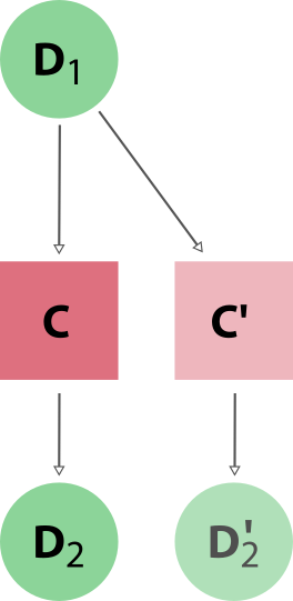
3.9. Saving compute time with caching#
Over the course of a project, you may end up re-running the same calculations multiple times - perhaps because two workflows include the same calculation.
Since AiiDA stores the full provenance of each calculation, it can detect whether a calculation has been run before and, instead of running it again, simply reuse its outputs, thereby saving valuable computational resources. This is what we mean by caching in AiiDA.
With caching enabled, AiiDA searches the database for a calculation of the same hash. If found, AiiDA creates a copy of the calculation node and its results, thus ensuring that the resulting provenance graph is independent of whether caching is enabled or not.
Caching happens on the calculation level (not the workchain level), and is not enabled by default.
We can enable it by setting the verdi config options.
%verdi config set caching.enabled_for 'aiida.calculations:quantumespresso.pw'
Success: 'caching.enabled_for' set to ['aiida.calculations:quantumespresso.pw'] for 'qe-to-aiida' profile
%verdi config list caching
name                     source    value
-----------------------  --------  -------------------------------------
caching.default_enabled  default   False
caching.disabled_for     default
caching.enabled_for      profile   aiida.calculations:quantumespresso.pw
Now, when we run the same calculation again, AiiDA will detect that it has already been run, and will simply reuse the results from the previous run!
output = aiida.engine.run_get_node(builder)
output.node
<CalcJobNode: uuid: 56d376de-9257-4d07-9b74-7eb3b9285151 (pk: 13) (aiida.calculations:quantumespresso.pw)>
We can see that the calculation was created from the cache by checking the following:
output.node.base.caching.is_created_from_cache
True
See also